11. Dataviz Code Session: Distribuições

11.1. Objetivos da DCS

• Aplicar técnicas de dataviz para plotagem e manipulação de representações visuais de distribuições.

• Elaborar RVs para dados de censo (Fonte: UCI ML Repository)

  • CSV disponível no kaggle.

11.2. Ferramentas utilizadas

• Módulos Python

  • pandas

  • matplotlib

  • seaborn

11.3. Aplicação do modelo referencial

• Vide Capítulo 3.

import pandas as pd
import seaborn as sb
import matplotlib.pyplot as plt

plt.style.use('../etc/gcpeixoto-datavis.mplstyle') # style sheet

11.3.1. Dados de entrada pré-processados

• Carregamento de dados

df = pd.read_csv('../data/adults.csv',skiprows=1)
df

	age	type-employer	fnlwgt	education	education_num	marital	occupation	relationship	race	sex	capital_gain	capital_loss	hr_per_week	country	income
0	39	State-gov	77516	Bachelors	13	Never-married	Adm-clerical	Not-in-family	White	Male	2174	0	40	United-States	<=50K
1	50	Self-emp-not-inc	83311	Bachelors	13	Married-civ-spouse	Exec-managerial	Husband	White	Male	0	0	13	United-States	<=50K
2	38	Private	215646	HS-grad	9	Divorced	Handlers-cleaners	Not-in-family	White	Male	0	0	40	United-States	<=50K
3	53	Private	234721	11th	7	Married-civ-spouse	Handlers-cleaners	Husband	Black	Male	0	0	40	United-States	<=50K
4	28	Private	338409	Bachelors	13	Married-civ-spouse	Prof-specialty	Wife	Black	Female	0	0	40	Cuba	<=50K
...	...	...	...	...	...	...	...	...	...	...	...	...	...	...	...
32556	27	Private	257302	Assoc-acdm	12	Married-civ-spouse	Tech-support	Wife	White	Female	0	0	38	United-States	<=50K
32557	40	Private	154374	HS-grad	9	Married-civ-spouse	Machine-op-inspct	Husband	White	Male	0	0	40	United-States	>50K
32558	58	Private	151910	HS-grad	9	Widowed	Adm-clerical	Unmarried	White	Female	0	0	40	United-States	<=50K
32559	22	Private	201490	HS-grad	9	Never-married	Adm-clerical	Own-child	White	Male	0	0	20	United-States	<=50K
32560	52	Self-emp-inc	287927	HS-grad	9	Married-civ-spouse	Exec-managerial	Wife	White	Female	15024	0	40	United-States	>50K

32561 rows × 15 columns

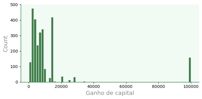
11.4. Visualização de distribuições univariadas

• Podemos usar seaborn.displot para plotagens gerais de distribuições:

  • kind = hist | kde | ecdf plotará histograma, ou kernel density estimation, ou ECDF

  • row e col expandem plots

  • A inclusão de y e hue gerará RVs similares a mapas de calor ou, proporções, quando hue for categórico.

dfa = df[df['capital_gain'] > 0]

# f é figure level
f = sb.displot(data=dfa,
           x='capital_gain',
           color='#005610', 
           edgecolor='w', 
           linewidth=1,
           kind='hist', # hist | kde | ecdf
           #row='race', # faz outros plots por linha
           #col='sex', # faz outros plots por colu
           #stat='density', # count | frequency | density | probability | percent | proportion           
           height=3.5, aspect=2 # aspecto usa proporção de altura
           )

# remover grid
for ax in f.axes.flat:
    ax.grid(False)
    ax.set_xlabel('Ganho de capital')

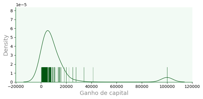
11.4.1. KDE e superposição

• Com kdeplot, temos a curva estimada por núcleos, a qual pode ser superposta ao histograma por meio de ax.

f2 = sb.kdeplot(data=dfa,
           x='capital_gain',
           color='#232a00',
           fill=False,
           alpha=0.9,
           ax=f.ax # habilite para sobrepor
           )

f2.grid(False)
f2.set_xlabel('Ganho de capital');

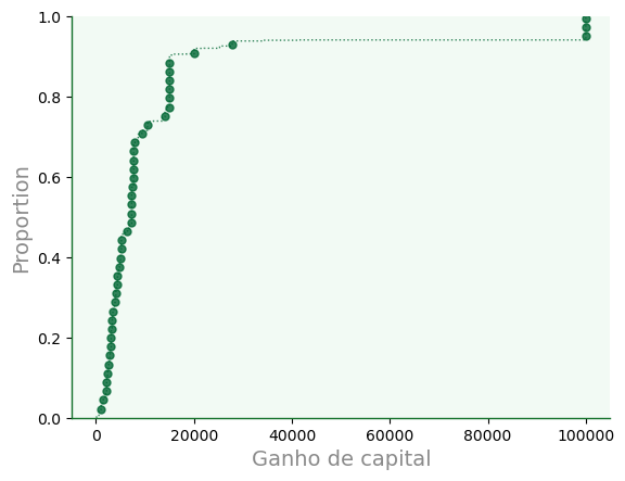
11.4.2. Distribuição cumulativa

• Distribuições cumulativas empíricas podem ser plotadas com ecdfplot.

f2a = sb.ecdfplot(data=dfa,
           x='capital_gain',
           color='#006633',
           alpha=0.8,
           linewidth=1.0,
           ls=':',
           marker='o',
           markersize=5,
           markevery=60
           #ax=f.ax # habilite para sobrepor
           )

f2a.grid(False)
f2a.set_xlabel('Ganho de capital');

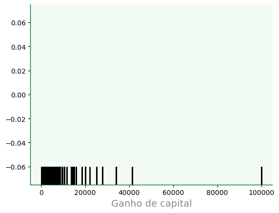
11.4.3. Plot tapete (ou borla)

• O rugplot é uma representação visual que adiciona traços similares a ticks no gráfico. O nome “rug” (tapete) deriva da lembrança de um tapete aberto com suas borlas (franjas) destacadas.

  • Também podemos construir rugs com a keyword rug em displot.

f3 = sb.rugplot(data=dfa,
           x='capital_gain',
           color='k',
           linewidth=2,
           height= 0.1, 
           )

f3.grid(False)
f3.set_xlabel('Ganho de capital');

11.4.3.1. Superposição de borlas

f4 = sb.displot(data=dfa,
           x='capital_gain',
           color='#005610', 
           linewidth=1,
           kind='kde',           
           height=3.5, 
           aspect=2,
           rug=True,
           rug_kws={
               'height': 0.2,
               'color': 'w',
               'linewidth': 0.5,
               'alpha': 0.5,
           }
           )

for ax in f4.axes.flat:
    ax.grid(False)
    ax.set_xlabel('Ganho de capital')

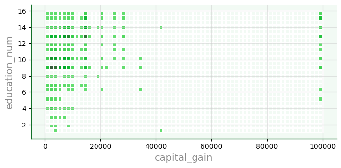
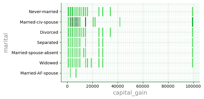
11.4.4. Outros visuais

• Mapa com displot

f5 = sb.displot(data=dfa,
           x='capital_gain',
           y='education_num',
           color='#005610', 
           edgecolor='w', 
           linewidth=1,
           height=3.5, aspect=2 # aspecto usa proporção de altura
           )

f6 = sb.displot(data=dfa,
           x='capital_gain',
           y='marital',
           color='#005610', 
           edgecolor='w', 
           linewidth=1,
           height=3.5, aspect=2 # aspecto usa proporção de altura
           )

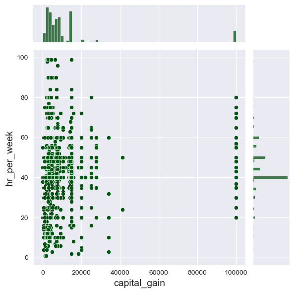
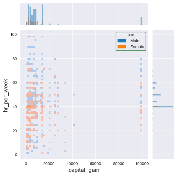
11.5. Distribuições bivariadas

• Usamos jointplot para exibir densidades a partir de relações entre duas variáveis.

  • Controle o tipo com kind e o hue

sb.set_style('darkgrid')
f7 = sb.jointplot(data=dfa,
           x='capital_gain',
           y='hr_per_week',
           color='#005610',
           height=6,     
           #hue='sex'
           kind='scatter' # 'scatter', 'hist', 'hex', 'kde', 'reg', 'resid']
           )

sb.set_style('darkgrid')
f7a = sb.jointplot(data=dfa,
           x='capital_gain',
           y='hr_per_week',
           color='#005610',
           height=6,     
           hue='sex',
           kind='hist' # 'scatter', 'hist', 'hex', 'kde', 'reg', 'resid']
           )

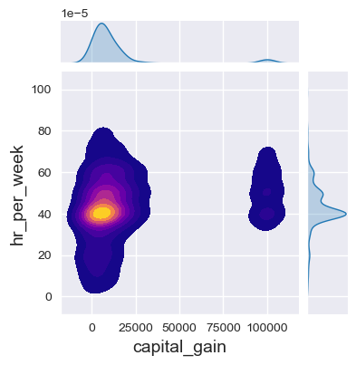
f7c = sb.jointplot(data=dfa,
           x='capital_gain',
           y='hr_per_week',
           height=4,     
           kind='kde', # 'scatter', 'hist', 'hex', 'kde', 'reg', 'resid'],
           fill=True,
           cmap='plasma'
           )

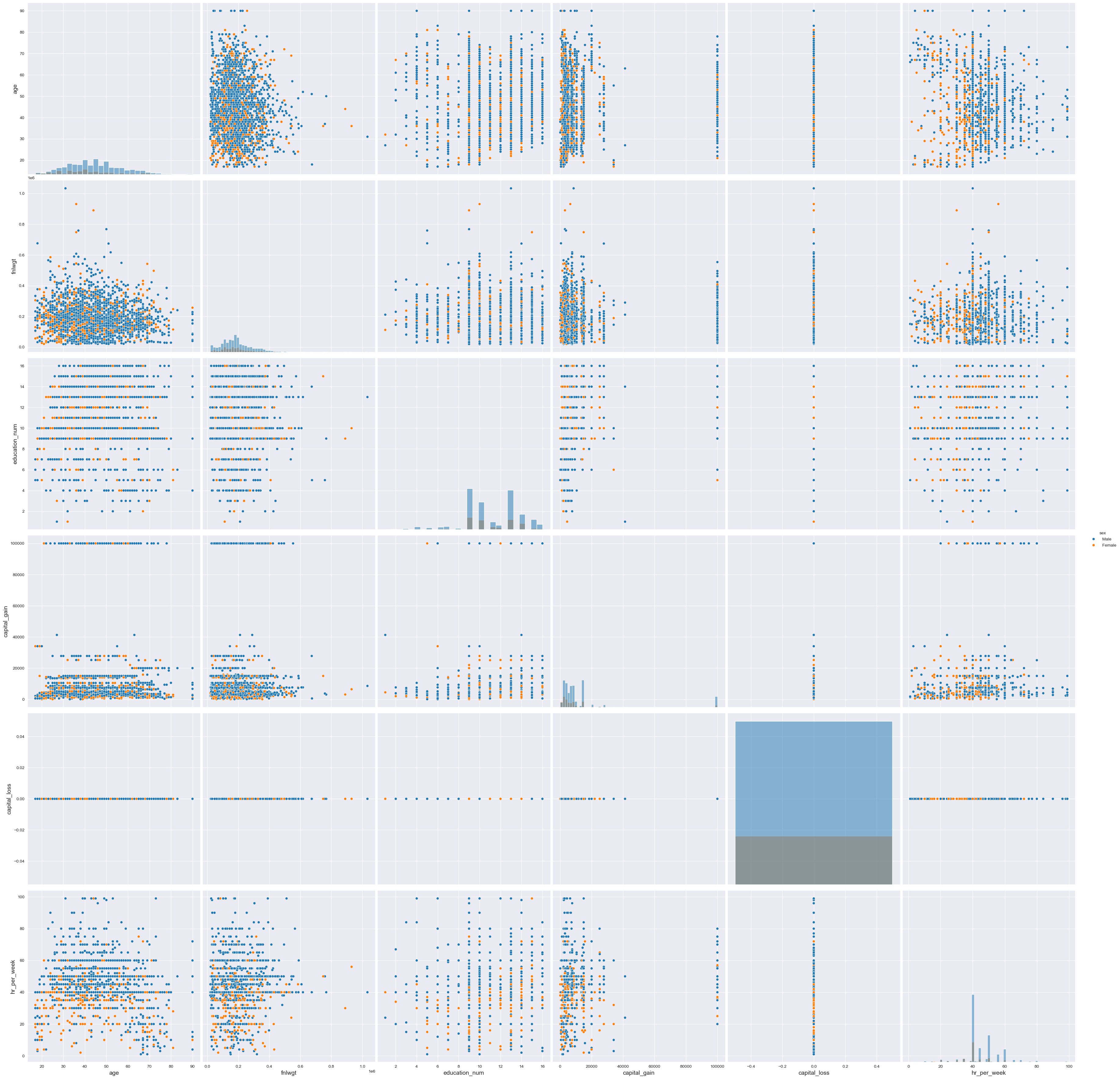
• Usamos pairplot para realizar plotagens de pareamentos em forma matricial

f7d = sb.pairplot(data=dfa,
           height=6,     
           hue='sex',
           kind='scatter', # 'scatter', 'hist', 'hex', 'kde', 'reg', 'resid'],
           diag_kind='hist'
           )