Este notebook explora aspectos do método da iteração linear, ou também chamado de método do ponto fixo.
import numpy as np
import matplotlib.pyplot as pltExemplo
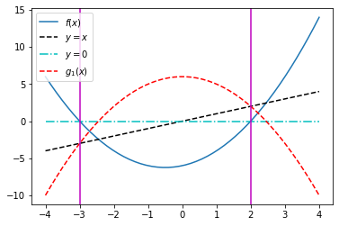
Estudamos a função .
x = np.linspace(-4,4,50)
f = lambda x: x**2 + x - 6

xr = np.roots([1,1,-6])
print('Raízes: x1 = {:f}, x2 = {:f}'.format(xr[0], xr[1]))

# função de iteração
g1 = lambda x: 6 - x**2

plt.plot(x,f(x),label='$f(x)$');
plt.plot(x,x,'k--',label='$y=x$');
plt.plot(x,0*x,'c-.',label='$y=0$');
plt.plot(x,g1(x),'r--',label='$g_1(x)$');

plt.axvline(-3,-5,10,color='m');
plt.axvline(2,-5,10,color='m');
plt.legend(loc='best');
Raízes: x1 = -3.000000, x2 = 2.000000
Exemplo
Estudamos a função
x2 = np.linspace(-1,1,50)

f2 = lambda x: np.exp(-x) - x
g2 = lambda x:  np.exp(-x)

plt.plot(x2,f2(x2),x2,g2(x2),'r',x2,x2,'c')
plt.grid(True)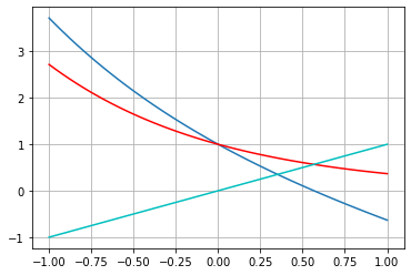
Implementação do método do ponto fixo
def ponto_fixo(x0,f,g,tol,N,vis):
    """
    Resolve problema de determinacao de raizes pelo
    metodo do ponto fixo (iteracao linear).

    entrada:

       x0  - aproximacao inicial        (float)
        f  - funcao a ser resolvida     (str)
        g  - funcao de iteracao         (str)
       tol - tolerancia                 (float)
        N  - numero maximo de iteracoes (int)
      vis  - flag para plotagem         (bool)

    saida:

       x   - raiz aproximada para f     (float)
    """
    from numpy import linspace
    from matplotlib.pyplot import plot,legend

    # funcoes
    f = eval('lambda x:' + f)
    g = eval('lambda x:' + g)

    # inicializacao
    it = 0 # contador
    x, xn = x0, x0 + 1 # iteradas atual, anterior

    e = abs(x-xn)/abs(x) # erro

    # tabela
    print('i\t x\t\t f(x)\t\t ER')
    print('{0:d}\t {1:f}\t {2:f}\t {3:e}'.format(it,x,f(x),e))

    # laco
    while e >= tol and it <= N:
        it += 1
        xn = x
        x = g(xn)
        e = abs(x-xn)/abs(x)
        print('{0:d}\t {1:f}\t {2:f}\t {3:e}'.format(it,x,f(x),e))

        if it > N:
            print('Solução nao alcancada com N iteracoes.')
            break

    if vis == True:
        dx = 2*x
        dom = linspace(x - dx,x + dx,30)
        plot(dom,f(dom),label='$f(x)$')
        plot(dom,dom*0,label='$y=0$')
        plot(dom,g(dom),label='$g(x)$')
        plot(dom,dom,label='$y=x$')
        legend()

    return x
Estudo de caso: 
Função de iteração:
f = 'x**2 + x - 6'
g = '(6 - x)**(1/2)'

x0 = 0.1
tol = 1e-5
N = 100

ponto_fixo(x0,f,g,tol,N,True)
i x f(x) ER
0 0.100000 -5.890000 1.000000e+01
1 2.428992 2.328992 9.588307e-01
2 1.889711 -0.539280 2.853771e-01
3 2.027385 0.137674 6.790695e-02
4 1.993142 -0.034243 1.718024e-02
5 2.001714 0.008572 4.282174e-03
6 1.999572 -0.002142 1.071346e-03
7 2.000107 0.000536 2.677864e-04
8 1.999973 -0.000134 6.694973e-05
9 2.000007 0.000033 1.673724e-05
10 1.999998 -0.000008 4.184321e-06
1.9999983262723453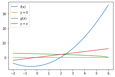
Função de iteração:
f = 'x**2 + x - 6'
g = '-(6 - x)**(1/2)'

x0 = 0.1
tol = 1e-5
N = 100

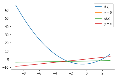
ponto_fixo(x0,f,g,tol,N,True)
i x f(x) ER
0 0.100000 -5.890000 1.000000e+01
1 -2.428992 -2.528992 1.041169e+00
2 -2.903273 -0.474281 1.633608e-01
3 -2.983835 -0.080563 2.699970e-02
4 -2.997305 -0.013469 4.493853e-03
5 -2.999551 -0.002246 7.488072e-04
6 -2.999925 -0.000374 1.247965e-04
7 -2.999988 -0.000062 2.079929e-05
8 -2.999998 -0.000010 3.466545e-06
-2.9999979200736955